Readability Scores Pt 1: Reference Guide

I started looking into readability scores in mid-October 2021, and the first thing that struck me was that there are a lot of readability scores. Most use similar methods to do the same thing, and most were verified in the same way. So, I’m compiling more a general overview and history of the more significant and interesting scores here ^{[footnote 1]}.

What is a readability score?

A readability score rates how difficult or easy a text is to read. They’re sometimes called formulas, indices, or measures; I’ll try to stick to “score” in this post, unless I’m giving the official name or quoting someone. A text can be pretty much anything: a chapter from a novel, an instruction manual, a website, a series of tweets, etc. The score itself is an equation that takes as input the text, calculates some features of the text (aspects of the text that can be turned into a number) and outputs a continuous number, sometimes rounded to the closest whole number.

Once you have a readability score, you have to verify that it is actually “correct”, that it predicts what it says it does. Most readability scores predict the grade level of a particular text, i.e. the earliest grade level at which you might expect a child to be able to read that text (which I do have some problems with, but that’s all in the next post). So, to verify the score most researchers do one of three things:

• grade texts using actual readers; if > 50% of a sample of 4th graders can read and correctly answer comprehension questions about the text, then that text is considered to be at a 4th grade reading level. Researchers then adjust the readability scores until it scores those texts to also be at a 4th grade level.
• make experts (teachers, learning professionals, book publishers) guess the grade level of texts, and adjust the readability score until it matches the guesses
• make their new score correspond to existing reading scores. Researches calculate the “relative rankings” of scores, i.e. scoring and ordering texts according to each readability score. They then try to end up with the same ordering of texts between the different scores.

Since most of these scores are equations, here are definitions of some commonly used variables in the scores:

• $ words $ is the total number of words in the whole text
• $ sents $ is the total number of sentences in the whole text
• $ sylls $ is the total number of syllables in the whole text

Simple Counts

Flesch Reading Ease

By far the most well known readability score (but not the most correct), the Flesch reading ease score is based on the average numbers of words per sentence and syllables per word. It was developed by Dr. Rudolf Flesch in the 1940’s.

The Flesch reading ease’s equation is:

\[206.835 - 1.015 ( \frac{words}{sents} ) \\ - 84.6 ( \frac{sylls}{words} )\]

Most readability scores around in the 40’s were intended for use with children. Teachers would use scores to decide if a text was the appropriate grade for a child: challenging but not disheartening. Flesch however developed his score to be used for adults. He tested it using the McCall-Crabbs Standard Test Lessons in Reading, which were passages graded by how well sample groups of children answered comprehension questions at the end of each passage.

Interestingly, at one point Flesh used the number of personal pronouns (I, you, etc.) and the number of affixes to words (“anti-“ in “antitoxin” and “-able” and “-ity” in “readability”) to compute the score. However, the people computing the score on new texts disregarded those features and only computed sentence length. As a result, Flesch split the score into two parts, the one known today, and another one known as the “human interest” score, which focused on the number of personal pronouns.

Nancy Ann Vieth’s MA thesis gives a great overview of Flesch’s development of the reading ease score, and the academic context at the time.

Flesch-Kincaid Grade Level Evaluation

Like the reading ease score, the Flesch-Kincaid grade level evaluation is based on the average numbers of words per sentence and syllables per word. It was co-developed by Flesch and J. Peter Kincaid in the 70’s for the US Navy.

The Flesch-Kincaid Grade Level Evaluation’s equation is:

\[-15.59 + 0.39 ( \frac{words}{sents}) \\ + 11.8 (\frac{sylls}{words})\]

The output is specifically the expected grade level of the text, which is why this equation looks to be the inverse of the reading ease score.

The grade level evaluation has more of an emphasis on shorter words, penalizing each additional average syllable per word 2.75 more than the reading ease. The Wikipedia user Cmglee made a good way to visualize this, shown below.

The grade level evaluation was validated using the Gates-MacGinitie Reading test.

Kincaid himself has some interesting thoughts on readability scores, particularly that they shouldn’t be over applied by writers, given how easy it is to game most of them.

If the read­ing level is too high, the easiest fix is to divide long sentences into shorter ones. This kind of chopping will indeed lower the readability level, but it’s often counter­ productive.

-Dr. J Peter Kincaid

Gunning Fog index

The Gunning Fog index was made by Robert Gunning, an American businessman in newspaper publishing, in 1952. His word to describe reading difficulty is “Fog”, thus the name, Gunning Fog. The score’s equation is:

\[0.4 \frac{words}{sents} + 100 \frac{complex\_words}{sents}\]

The output is the grade level of the text. Complex words are words that have more than 3 syllables, not including several common syllables such as -ing.

It requires a minimum of 100 words in the text when calculating the score. It is important to note that most scores developed before 1990 were standardized and validated on longer prose, at least a paragraph or two of text. The scores that you get with shorter amounts of text are less likely to be the true readability of the text. This fact makes it difficult to apply the more commonly used readability scores to shorter amounts of text that you would find on a webpage, or in a tweet.

Fry Readability Graph

The Fry Readability Graph, developed by Edward Fry in 1968, is pretty straight forward.

1. Sample several 100 word groups from the text
2. Calculate the number of syllables and sentences in those groups
3. Use those calculations to place a point on a “graph” (aka a plot with word length on the x-axis and average number of sentences on the y-axis).

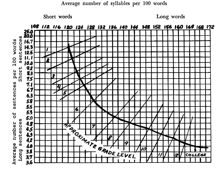
It was validated using “a lot of” book publisher grade level recommendations. The lack of an actual equation, deferring to the flexible but approximate graph, probably didn’t help the score’s usage.

However, Fry does tell us why some many readability scores were developed in the 1950’s - early 80’s:

Though readability formulas are used by some teachers, some librarians, and some publishers, their number is all too few. Perhaps the sheer time it takes to apply these formulas causes them mostly to languish in term papers and occasional magazine articles.

SMOG (Simple Measure of Gobbledegook)

G. Harry McLaughlin, the Editor at the Mirror newspaper and Doctor of Psycholinguistics at University of London, published his SMOG score at the University of Syracuse in 1969. Sold as a simpler version of the Fry Readability Graph, it consists of three steps:

1. Count sentences (at least 30)
2. Count polysyllables (>=3 syllables)
3. \(1.043 \sqrt{polysyll (30 / sents)} \\ + 3.1291\) gets you the grade level.

An even simpler approximation of the last step is to take the square root of the nearest perfect square of the number of polysyllables. So if there are 95 polysyllables in the sample, you round to 100, and take the square root, which means the text is at a 10th grade level.

McLaughlin also suggests that the text be at least 30 sentences (which he estimates to be 600 words), saying that a sample of 100 words “is so small that it may be quite uncharacteristic of the text being assessed.”

ARI (Automatic Readability Index)

The Automatic Readability Index (1967) is unique in this list because it was created in mind with real time type-writer readability monitoring. To do that in the 60’s, they used characters per word instead of the usual syllables per word.

\[4.71 \frac{characters}{words} \\ + 0.5 \frac{words}{sents} - 21.43\]

Word Lists

All of the scores above tend to reduce text to two, maybe three numerical features such as syllable or word counts, and don’t consider the content of the text. Word lists attempt to fix this problem. They still reduce the text to some number, but this time if you changed every letter in every word, it would make a difference to the readability score.

The two methods worth listing here are Thorndike’s word list, and the Dale-Chall readability formula.

Thorndike’s word list, first published in 1921, has about 20,000 words now, and isn’t exactly a readability measure on it’s own, but forms the basis of other readability scores based on word lists. Thorndike’s word list is mainly ordered by frequency of words in texts, and by assumption, familiarity.

The Dale-Chall formula was developed by Edgar Dale and Jeanne Chall in 1948. It used a list of 763 words that 4th grader were familiar with, and in 1995, was updated to include 3000 familiar words. Assuming that any word not on the list is considered to be a hard word, the equation is:

\[0.1579 (\frac{hardwords}{words} * 100) \\ + 0.0496 (\frac{words}{sents})\]

These methods were generally used before the above counting methods were invented, and besides for Dale-Chall, they aren’t talked about much anymore. Some criticism of them were that:

• the lists were too long to use by hand, which is a valid argument in 1940. Reading through an 8 page list for every word in the text is very tiresome (though I can’t tell how long some of those word lists got to be). Nowadays, this argument is less useful, as there’s no meaningful performance difference on modern computers between doing O(N) set existence queries vs simple counts.
• the lists were very influenced by what materials the words were counted from. This is a valid point, and one that is still important today.
• the lists only show familiarity with the words, as words can still be abstract, ambiguous, or vague, depending on the context in which they’re used.

Multi-feature Methods

It might stand out that all of the readability scores above were created a while back: the latest is the Flesch-Kincaid score, from 1975. Computing power, especially with regards to text and natural language processing (NLP), has significantly increased since the 70’s, as has the prevalence of personal computers. With the development of NLP as a field in artificial intelligence, new methods have been used to compute readability scores. For the purposes of naming them, we’ll call these methods multi-feature methods.

The key difference between multi-feature methods and the methods above are that multi-feature methods generally rely on many more features of the text. While scores like Dale-Chall and SMOG rely on 2 or 3 different features of the text like the number of sentences and the complexity of each word, multi-feature methods rely on many more features, including grammatical analysis, named entity counts, and deep-learned features. Due to the high number of features, these methods need to be trained on specific datasets, sometimes called a corpus. This allows them to be more specific to a particular type of text, like texts from the healthcare or legal industries, though overfitting should be avoided.

Training on specific corpuses can get around a lot of the downsides mentioned in the word lists section. The lists can’t get too long; that complexity is handled by the algorithm.

Collins-Thompson Callan Score

The Collins-Thompson-Callan score, introduced in 2004 in this paper, outlined the basic gist of a multi-feature readability score algorithm:

• gather a specific corpus of texts. Since the authors of this paper wanted to make a readability score made for web pages, they found 550 documents, each marked to a certain reading level grade by the website authors.
• use a variant on a naive bayes classifier to predict the “class” (the reading grade level) based on the presence of certain words. Since each word in a document is considered without it’s surrounding context, i.e. one word at a time, the authors call it a unigram model.
• Smooth it: the training words are smoothed across grade levels, across the language model (using Simple Good-Turing smoothing), and the final resulting grade level is the average for the top 2 predicted grades.

Specific Target Audiences

All of the above readability scores try to target their output to the most people possible. However, not everyone struggles with reading comprehension for the same reasons. Grade school students have different challenges with reading than people who are learning english as a second or third language, and people with intellectual disabilities have different challenges than either of those groups. Lumping these groups together to try to predict a single readability score isn’t going to be the most accurate for the groups individually. The next few scores, despite using different methods (counts vs multi-feature), target one of these subpopulations.

McAlpine EFLAW Readability Score

The McAlpine EFLAW score was made specifically for “Global English for Global Business”. The name is a combination of “EFL”, or “English as a Foreign Language”, and “flaw”, or flaws of writing for an English as a foreign language audience. It’s based on the idea that English learners have more trouble with clusters of shorter words of 1-3 letters, called miniwords. A phrase like “In relation to the date of a new time”, would have 7 miniwords.

The score isn’t normalized to grade levels, but it still increases as its difficulty does.

\[(words + miniwords) / sents\]

Multi-Feature Scores for EFL Learners

The LXPER Index 2.0 is a “text readability assessment model”, built to work for non-native language learners (specifically Korean), similarly to the McAlipne EFLAW score above. However, it’s specifically targeted at texts in “foreign English language training curriculums”. The reading levels are targeted to grade levels so that texts will properly challenge students and improve their language learning. Additionally, it takes into account that student’s primary interaction with the language they are learning is through the curriculum. Word lists like Dale-Chall and other readability scores assume that the reader will have broad and diverse exposure to the target language, but foreign language learners not immersed in the language will have a much more limited exposure.

This method is a multi-feature readability score. Several dozen different text features, including many of the ones mentioned in other readability scores like average words per sentence and percentage of “complicated” words are all included, as well as more detailed features such as the average number of verb phrases and other grammatical structures in the text, the number of entities and lexical chains in the text, and the number of pre-graded vocabulary words. All of these features are used in a logistic regression model, which is trained on pre-graded text samples.

Intellectual Disabilities

Some more advanced scores attempt to find more features that are directly correlated to readability, like Feng, Elhadad, and Huenerfauth. Those authors focus on readability for people with intellectual disabilities, which gives some valuable insights into the actual process of readability that most readers subconsciously work with each time they read.

Notable from the above paper is that entity density is important. Entity density is the number of things mentioned in a sentence, and how many times they were mentioned; essentially, how much your working memory is used when reading. Earlier studies with the intellectually disabled population showed that “these users are better at decoding words than at comprehending text meaning.” So reading longer words isn’t super hard, but trying to create a “cohesive representation of discourse” can be. They also found was that “texts designed for children may not always lead to accurate models of the readability of texts for other groups of low-literacy users”. That insight is important for readability scores in general: most were made specifically for children grade levels!

Misc Readability scores

Other readability scores that I found in my research, but didn’t write about here.

• Spache
• Botel
• Coleman-Liau, also uses characters per word
• Linsear Write
• LIX (Läsbarhetsindex), one of the few tests developed outside of the US, in Sweeden
• Xia et al., 2016, another multi-feature approach for EFL

So, what now?

So now that we know about many readability scores, what should we do with them? Which ones should we use, and which ones should we avoid? I try to address some of those question in part 2 of this blog